Adopting the Quadratic Mean Process to Quantify the Qualitative Risk Analysis
Publications
PMI Global Congress 2013 – North America
New Orleans – Louisiana – USA – 2013
Abstract
The objective of this paper is to propose a mathematical process to turn the results of a qualitative risk analysis into numeric indicators to support better decisions regarding risk response strategies.
Using a five-level scale for probability and a set of scales to measure different aspects of the impact and time horizon, a simple mathematical process is developed using the quadratic mean (also known as root mean square) to calculate the numerical exposition of the risk and consequently, the numerical exposition of the project risks.
This paper also supports the reduction of intuitive thinking when evaluating risks, often subject to illusions, which can cause perception errors. These predictable mental errors, such as overconfidence, confirmation traps, optimism bias, zero-risk bias, sunk-cost effect, and others often lead to the underestimation of costs and effort, poor resource planning, and other low-quality decisions (VIRINE, 2010).
Qualitative X Quantitative Risk Analysis
One of the main challenges during the analysis of a risk is to define the right approach to assess the amount of the exposure/opportunity. The two basic steps to determine the right level of risk are based on the qualitative and quantitative analysis (Exhibit 1).
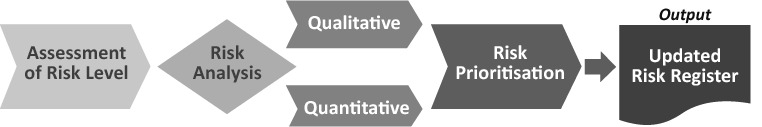
Exhibit 1 – Analysis of Risk Process Flow (ROSSI, 2007).
A qualitative risk analysis prioritizes the identified project risks using a predefined scale. Risks will be scored based on their probability or likelihood of occurrence and the impact on project objectives if they occur (Exhibit 2 and 3).
Level | Score | For Threats | |
Exhibit 2 – Example of scales used in the qualitative risk analysis | |||
High | Very High | 5 | Red |
High | 4 | ||
Medium | Medium | 3 | Yellow |
Low | 2 | ||
Low | Very Low | 1 | Green |

Exhibit 3 – Example of Qualitative Risk Matrix with 3 x 3 Levels (ALTENBACH, 1995)
A quantitative risk analysis is based on simulation models and probabilistic analysis, where the possible outcomes for the project are evaluated, providing a quantitative, numeric and many times financial risk exposure to support decisions when there is uncertainty (PMI, 2013). Some quantitative processes are simple and direct like rolling a dice (Exhibit 4), but most of them involve very complex simulation scenarios like the Monte Carlo Simulation.
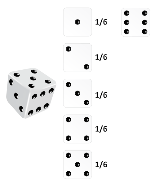 Exhibit 4 – Diagram showing the deterministic probability of rolling a dice
“Monte Carlo” was a nickname of a top-secret project related to the drawing and to the project of atomic weapons developed by the mathematician John von Neumann (POUNDSTONE, 1993 and VARGAS, 2013). He discovered that a simple model of random samples could solve certain mathematical problems, which couldn’t be solved up to that moment.
The simulation refers, however, to a method by which the distribution of possible results is produced from successive recalculations of project data, allowing the development of multiple scenarios. In each one of the calculations, new random data is used to represent a repetitive and interactive process. The combination of all these results creates a probabilistic distribution of the results (Exhibit 5 and 6).
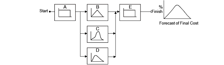
Exhibit 5 – Construction of model of distribution of costs and activities or work packages making up a final distribution from random data of the project (PRITCHARD, 2001).
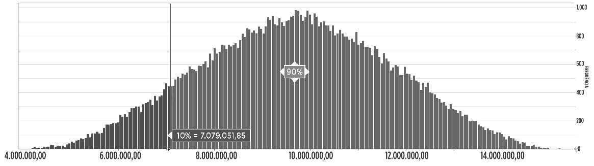 Exhibit 6 – Example of Monte Carlo simulation to assess the cost impact of a potential threat to the project
Because quantitative analysis is based on mathematics and statistics supported by objective metrics, such analyses are considered to be more rigorous (SMOCK, 2002). The main challenges of a solid quantitative analysis are the time and effort it requires to be executed and the required technical background in statistics to make the proper parameterization of the data. The main advantages and disadvantages of each method are presented in the Exhibit 7.
Quantitative Methods | Qualitative methods | |
Exhibit 7 – Example of Monte Carlo simulation to assess the cost impact of a potential threat to the project (based on ROT, 2008) | ||
Advantages | Facilitates the cost benefit analysis Gives a more accurate value of the risk More valuable | Relatively simple to be implemented Easily determine risk categories with greater impact in the project Visually impactful |
Disadvantages | Results of the method may not be precise Numbers can give a false perception of precision More expensive and time consuming | A lack of understanding of the parameters used in the scale can lead to different interpretations Results can be biased Less valuable |
The risk model proposed hereafter is a qualitative process with numerical results, reducing the ambiguity of the qualitative process without adds the time and effort to determine with precision the probability and the impact of uncertain events in the project.
Assessing Probability
The proposed qualitative probability assessment is based on a scale with their respective scores (Exhibit 8).
Level | Score | Description | |
Exhibit 8 – 5 Scales to assess the risk probability | |||
| Very High | 5 | It is expected that the event will occur. If it does not occurs it will be a surprise. |
High | 4 | The event has a great chance of occurring. | |
Medium | 3 | The event can occur. | |
Low | 2 | It will be a surprise if the event occurs. | |
Very Low | 1 | Very remote chance of the event to happen. Practically impossible. | |

For each identified risk a score from 1 (one) to 5 (five) should be determined.
5 Dimensions of the Impact
The impact of the event, in case it occurs, can be perceived in different dimensions of the project objectives. For example, one risk can have a major impact on costs but not necessarily an important impact in quality. It is very important to highlight that threats and opportunities should be analyzed separately.
The basic groups where impact should be evaluated are (Exhibit 9):
- impact on time and deadlines
- impact on costs
- impact on quality
- impact in safety and security
- other impacts
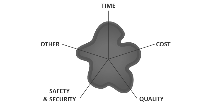
Exhibit 9 – Basic impact groups showing the different impact dimensions of one specific risk
Each project may develop different impact groups based on the nature of the project, including groups like: impact on reputation, regulatory impact, environmental impact, social impact, and stakeholder’s impact, among several others. Following is the presentation of the 5 basic groups.
Impact on Time and Deadlines
One should assess the level of impact on the conclusion of the project. It can be positive or negative for opportunities and threats, respectively. Threats that impact the conclusion of the project must be considered as a priority if compared to other events.
Because each project differs in size, complexity and several other factors, the project team needs to agree on the level of tolerance that they consider appropriate for each level of impact, like the example shown in Exhibit 10.
Level | Score | Description | |
Exhibit 10 – Example of impact scale and score for time and deadlines | |||
| Very High | 5 | Delays/Anticipation above 180 days or 6 months. |
High | 4 | Delays/Anticipation between 120 and 180 calendar days. | |
Medium | 3 | Delays/Anticipation between 60 and 120 calendar days. | |
Low | 2 | Delays/Anticipation between 15 and 60 calendar days. | |
Very Low | 1 | Less than 15 calendar days of delays/anticipation. | |

Impact on Costs
One should also assess the level of impact that the event may bring to the total project cost. It can be positive (savings) or negative (additional expenditures) for opportunities and threats, respectively.
Like mentioned for time and deadlines, the project team needs to agree on the level of tolerance that they consider appropriate for each level of impact, like in the example for costs presented in the Exhibit 11.
Level | Score | Description | |
Exhibit 11 – Example of impact scale and score for costs | |||
| Very High | 5 | Variation (positive or negative) above $1,000,000. |
High | 4 | Variation (positive or negative) between $500,000 and $1,000,000. | |
Medium | 3 | Variation (positive or negative) between $250,000 and $500,000. | |
Low | 2 | Variation (positive or negative) between $100,000 and $250,000. | |
Very Low | 1 | Variation (positive or negative) lower than $100,000. | |

Impact on Quality
Assesses the level of impact on the quality required for the project. It can be positive or negative for opportunities and threats, respectively.
As presented in the other groups, the project team needs to agree on the level of tolerance that they consider appropriate for each level of impact like in the example in Exhibit 12 for negative risk events.
Level | Score | Description | |
Exhibit 12 – Example of impact scale and score for quality (only negative events) | |||
| Very High | 5 | Client rejects the delivery or product. |
High | 4 | Client asks for immediate corrective actions. | |
Medium | 3 | Client perceives and asks for action/information. | |
Low | 2 | Client perceives but forgives and no action is needed. | |
Very Low | 1 | Imperceptible impact (most of the time not even perceived by the stakeholders). | |

Impact in Safety and Security
Assesses the level of impact that the event can incur in safety at work and security. This impact group could include or not aspects related to environment, physical security of the work in the project, data security (IT), and reputation, among others.
In the Exhibit 13, an example of scale is presented to assess impacts in safety and security.
Level | Score | Description | |
Exhibit 13 – Example of impact scale and score for safety and security, with focus in environment and reputation | |||
| Very High | 5 | Crisis. Impact is so evident and public that the project could not proceed as planned. |
High | 4 | Evident impact on environment/reputation. | |
Medium | 3 | Impact is perceived and raises concerns. | |
Low | 2 | Perceived impact on environment/reputation but without relevance. | |
Very Low | 1 | No impact on environment and reputation. | |

Other impacts
This group is an optional group and aims to include any other specific impact of a risk that was not covered in the previous groups. It is important that the score of the other impacts, if it exists, should be from 1 to 5 like the other impact groups.
Proximity: The 6th Impact Dimension
Another dimension of the impact is the time horizon or proximity of the event (Exhibit 14). An event that may happen in hours requires different actions than another event that could impact the project in 2 years. If an event is close to happen, it has a higher priority if compared with future events (in the proximity aspect).
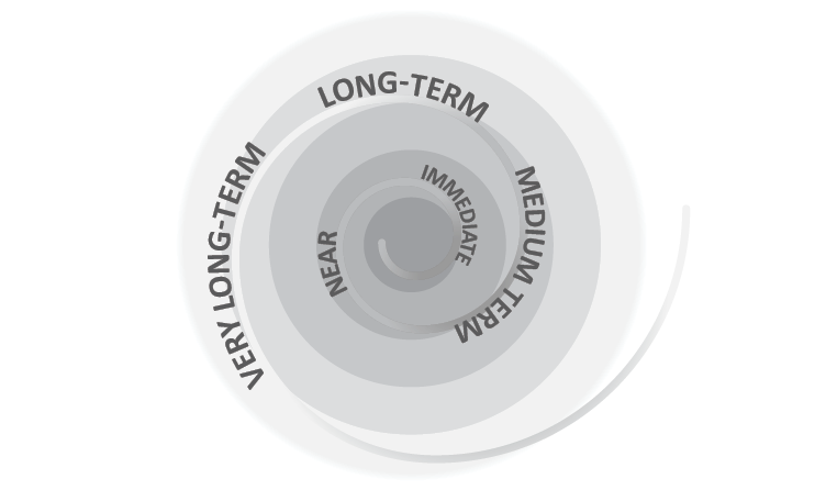
Exhibit 14 – Understanding the time horizon
The proximity scale should be compatible with the other impact groups (1 to 5 score for different time horizons). It is important that the project team defines what are immediate events, short-term events, medium-term events, long-term events and very long-term events (Exhibit 15).
It is important to highlight that immediate events will score higher than very long-term events when assessing their proximity.
Level | Score | Description | |
Exhibit 15 – Example of proximity scale and score | |||
| Very High | 5 | Event can happen anytime in the next 15 days. |
High | 4 | Event can happen between 15 days and 3 months. | |
Medium | 3 | Event can happen between 3 and 6 months. | |
Low | 2 | Event can happen between 6 months and 1 year. | |
Very Low | 1 | Event can happen more than 1 year ahead. | |

Calculating the expected value and final risk assessment
The expected value is a risk measurement used to assess and prioritize risk events (Exhibit 16).

Exhibit 16
Using the qualitative method, the probability will range from 1 to 5 (Exhibit 8).
The impact is based on the impact in different aspects of the project and the proximity using a quadratic mean (root square mean) calculation (Exhibit 17).
 Exhibit 17
The decision for the quadratic mean instead of the arithmetic mean is based on the concept that different levels of impact add additional exposure to the project and this variance should be considered as a risk factor to the project.
The relationship between the quadratic mean and the arithmetic mean is

Exhibit 18
where the variance is a measure of how far a set of numbers is spread out
The variance concept is directly related to the dispersion of the different impact groups. If the impact ranges are very wide, the variance will also be high and the difference between the proposed quadratic mean and the traditional arithmetic mean will increase, increasing the risk impact.
One example of the impact results is presented in the Exhibit 19.
Impact Time | Impact Cost | Impact Quality | Impact S&S | Other Impact | Proximity | |
Risk A | 3 | 2 | 1 | 1 | 1 | 4 |

Exhibit 19
It is important to highlight that the threats and opportunities can be calculated using the same formula, but with different signals (+ for opportunities and – for threats). The total qualitative risk exposure of the project is determined by the sum of the expected values of all threats and opportunities. An example of this process is presented on the Exhibit 20.
Type | Proba- bility | Proxi- mity | Impact Time | Impact Cost | Impact Quality | Impact Safety and Security | Other Impacts | Total Impact | Expected Value |
Total Risk Expected Value | (5,10) | ||||||||
Exhibit 20 – Example of a project expected risk value considering opportunities and threats. | |||||||||
Threat | 1 | 3 | 2 | 1 | 1 | 1 | 4 | 2,31 | (2,31) |
Threat | 2 | 4 | 4 | 3 | 3 | 4 | 3 | 3,54 | (7,07) |
Threat | 2 | 3 | 5 | 4 | 4 | 5 | 1 | 3,92 | (7,83) |
Opportunity | 3 | 2 | 4 | 3 | 5 | 4 | 2 | 3,51 | 10,54 |
Opportunity | 4 | 1 | 3 | 2 | 4 | 3 | 2 | 2,68 | 10,71 |
Threat | 5 | 2 | 2 | 1 | 3 | 1 | 1 | 1,83 | (9,13) |
The results from the process will be always a number between 1 and 25. In the example of Exhibit 20, the value -5,10 is equivalent to 20,4% negative exposure (5,10/25) for the Project.
Based on this result and the tolerance thresholds (HILSON & MURRAY-WEBSTER, 2007), the total exposure can be compared with other projects and the corporate limits to define potential risk response plans.
Conclusions
The qualitative risk method is always a simplified model if compared with the quantitative methods. The approach of this paper suggests an alternative model that can be tailored to include different kinds of impacts and scales in order to produce a reliable quantitative result.
This result allows opportunities and threats to be compared in order to determine the total risk exposure. The concept that an opportunity can cancel a threat of the same level is not possible with the traditional qualitative risk management approach.
References
ALTENBACH, T. J. (1995). A Comparison of Risk Assessment Techniques from Qualitative to Quantitative. Honolulu, ASME Preassure Vessels and Piping Conference. Available at http://www.osti.gov/bridge/servlets/purl/67753-dsZ0vB/webviewable/67753.pdf
HILSON, D. & MURRAY-WEBSTER, R. (2007). Understanding and Managing Risk Attitude. London: Gower Publishing.
PMI (2013). The Project Management Body of Knowledge: Fifth Edition. Newtown Square: Project Management Institute.
POUNDSTONE, W (1993). Prisoner’s Dillema. Flushing: Anchor Publishing Group.
PRITCHARD, C. L. (2001). Risk Management: Concepts and Guidance. 2ª Ed. Arlington: ESI International.
ROSSI, P. (2007). How to link the qualitative and the quantitative risk assessment. Budapest: Project Management Institute Global Congress EMEA.
ROT, A. (2008). IT Risk Assessment: Quantitative and Qualitative Approach. San Francisco: World Congress on Engineering and Computer Science.
SMOCK, R. (2002). Reducing Subjectivity in Qualitative Risk Assessments. Bethesda, SANS Institute. Available at http://www.giac.org/paper/gsec/2014/reducing-subjectivity-qualitative-risk-assessments/103489
VARGAS, R. V. (2013). Determining the Mathematical ROI of a Project Management Implementation. New Orleans, Project Management Institute Global Congress North America.
VIRINE, L. (2010). Project Risk Analysis: How Ignoring It Will Lead to Project Failures. Washington: Project Management Institute Global Congress North America.
Risk Management , Risk , Residual Risks , Secondary Risks , Risk Responses